NaClhv

Now, what kind of data do we have to determine the shape parameter?

We have the historical data, of course. We have some number of people who are said to have been resurrected in some sense, and each of these people has some amount of evidence associated with their resurrection claim.

We essentially want to "fit" these evidence data into a generalized Pareto distribution, and read off the shape parameter. However, this will be somewhat tricky. We do not have the complete data for all 1e9 reportable deaths throughout human history. We can reasonably assume that the vast majority of them would have essentially zero evidence for a resurrection, but the complete data set would be pretty much impossible to obtain. We don't even have the complete data set just for the outliers - cases like Apollonius or Zalmoxis, where there is a distinctly non-zero level of evidence for a resurrection. Furthermore, the precision on determining the level of evidence is rather poor. All this means that the usual "fit a curve through some kind of x-y scatterplot" approach would not work very well.

However, given that we already know we'll be fitting a generalized Pareto distribution, this is not necessary. We're just looking for the shape parameter, and for that, we merely need to count the number of outliers near the maximum value. Consider the following graph:

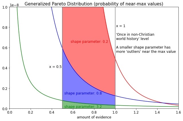
This is the same graph as before, in the sense that it just shows the generalized Pareto distribution, scaled so that the probability of x > 1 is 1e-9. Once again, this means that the maximum evidence from 1e9 reportable deaths is likely to appear around x = 1.

However, we now want to focus on how to fit the data. And since the data will have x values less than the maximum, this graph is scaled so that we're focusing to the left of the x = 1 line, instead of the tail to the right.

In particular, note the vast differences in the area under the curve for different shape parameters. The shaded regions represent the probability of finding an "outlier" - a non-Christian resurrection report with at least 20% of the evidence of the maximum report. For instance, the reports of the resurrection of Puhua or Apollonius would be considered an "outlier".

So, let's look at the green curve, with a shape parameter of 20, and a tiny area under the curve. If this were the skeptic's distribution, you'd expect essentially no other outliers. The maximum value would stand by itself, with no other outliers coming anywhere near its value.

Similarly, if the shape parameter is 2, you'd expect perhaps one outlier out of 1e9 samples - one other resurrection report would have at least 20% of the evidence of the maximum.

Lastly, if the shape parameter is 0.2, you'd expect many, many outliers. The probability distribution grows very rapidly as it goes backward from x = 1, and therefore you expect to find many other resurrection reports with a similar level of evidence as the maximum.

So by counting the number of outliers, we can make a determination about the shape parameters.

But... wait a minute. Having more outliers is associated with smaller shape parameters? But didn't smaller shape parameters correspond to a faster-decaying function, and therefore a lower probability for the "skeptic's distribution" generating a Jesus-level of evidence? Wouldn't this lead to the "skeptic's distribution" being less able to explain the evidence for Jesus's resurrection, and therefore make the resurrection more likely?

Are we saying that having MORE non-Christian resurrections reports (like Apollonius or Zalmoxis) make Jesus's resurrection MORE likely?

That is precisely what we are saying. The following analogy may help understand how this could be.

Alice accuses Bob of theft. Bob is known to have come into a sudden possession of $100,000. He is also known to be a gambler. He claims that his sudden fortune came from a lucky night at the card table, but Alice believes that he stole the money - she claims that $100,000 is far too large a sum for Bob to have naturally won through gambling. 

Carol takes on this investigation. She looks into Bob's past gambling history, to see it's realistic for him to have won $100,000 in a single night. She finds that, among Bob's past verifiable winnings, there were two nights where Bob won $5,000 and $3000. These are his most remarkable winnings on record, and Carol cannot find any other instances where he won more than $1000 on a single night. 

Carol concludes that she does not really have enough information. It could be that Bob plays a card game with an erratic payout scheme, where winning 20 or 30 times more money is not that unusual. Maybe it has some kind of "let it ride" or "double or nothing" mechanism which makes such returns plausible. Or maybe Bob himself is an erratic gambler, and decided to bet a lot more money that one night to win the $100,000. Based on all this, Carol decides to be skeptical of Alice's claim that Bob stole the money. Her own "skeptic's distribution" for how much money Bob can win does not decay quickly enough. There are relatively few outliers near his maximum winnings of $5000, and this suggests that it decays very slowly - meaning that the $5000 cannot be established as a limit to what Bob can win. His theoretical winnings can possibly stretch quite far into the higher values, making it impossible to rule out a $100,000 winning. 

But then, Carol has a breakthrough in her investigation. She finds extensive, previously undiscovered records of Bob's gambling winnings, and it shows that Bob has won more than a $1000 on dozens of nights. The maximum that he's won is still $5000, but he's also regularly won thousands of dollars in a single night. 

Carol takes this new information into account, and adjust her "skeptic's distribution" for how much Bob can win in a single night. Clearly, Bob's winnings are not erratic; he regularly wins up to about $5000. But this also establishes, with the weight of those repeated winnings, that this is close to the likely upper limit for what he can win in one night. 

Carol therefore decides to believe Alice. Her "skeptic's distribution" cannot explain how Bob would naturally win $100,000 in a single night, because it goes against his established pattern of regularly winning up to $5000. She pursues the case further, and eventually convicts Bob of theft.

This is not just a story; it can be mathematically established, and it will be in the future posts. For now, this story just provides the intuitive backing for the mathematical results to come.

So, having more non-Christian reports of a resurrection, with their pathetically low levels of evidence behind them, only make Jesus's resurrection more likely. When skeptics say "don't you know there are numerous other Jesus-like stories of someone dying and resurrecting?", they are only kicking against the goads. The more numerous such cases they come up with, the more firmly it establishes that Jesus really did rise from the dead.

The next post will bring the last several posts together, to fully spec out the program which will compute the complete "skeptic's distribution", from which we can calculate its chances of predicting a Jesus-level of evidence for a resurrection.

You may next want to read:
Christmas and time
For Christmas: the Incarnation
Another post, from the table of contents